Star Plots
Simulations of the Night Sky
I love looking at a starry night sky. For me it's uniquely awe-inspiring and meditative. Clouds, the Moon, light pollution, responsibilities, even laziness, all work against my seeing it. On the relatively rare occasions when I get out under a truly dark sky, I'm usually anxious to make the most of it, but sometimes I get tired of fiddling with telescopes and observing lists, and I just want to lie in the grass and stare at the sky.
A long time ago, I started working on a LightWave plug-in that renders the million or so (now 2.4 million) stars in the Tycho catalog. There are obvious practical reasons for a space visualizer to have a good starfield tool, but all of that, including the space visualizer part, came much later. I started out with the simple desire to paint what I love in a medium I understood.
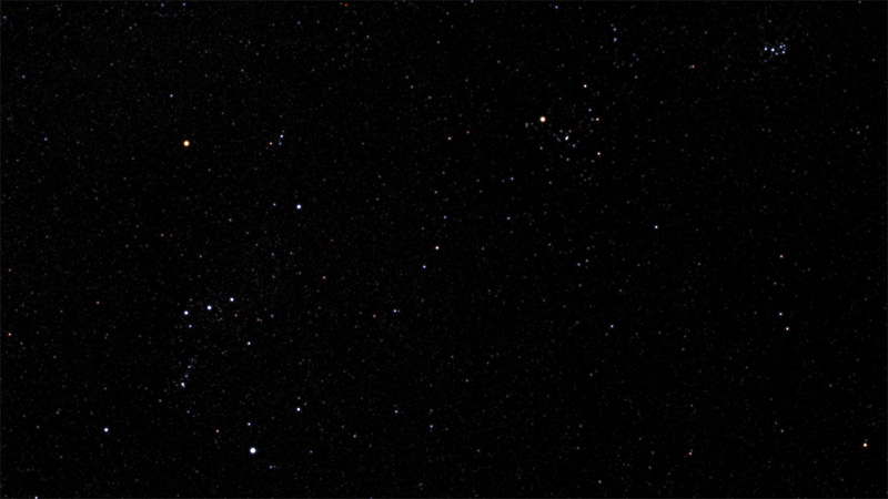
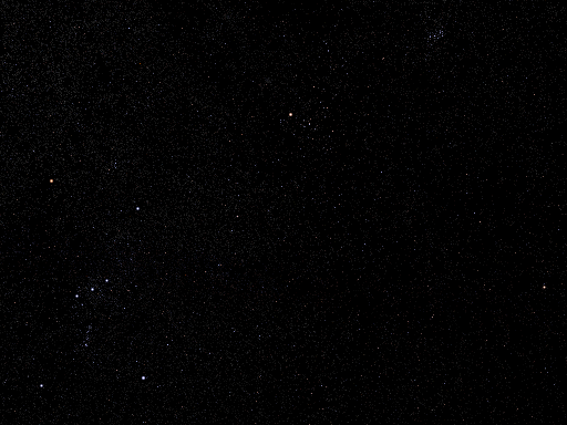
Orion and the Hyades and Pleiades star clusters in Taurus, visible during northern hemisphere winter. The crazy red star at the top edge is 119 Tauri, the second-reddest bright star after Herschel's Garnet Star, Mu Cephei.
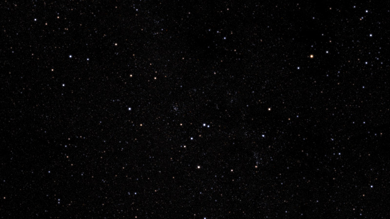
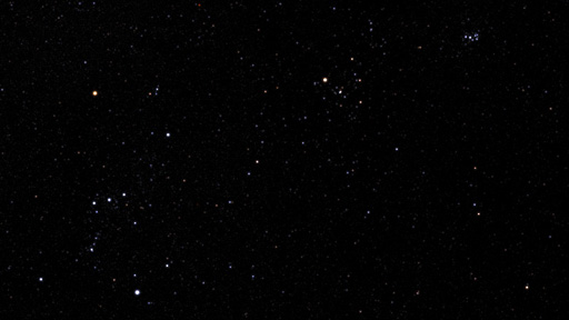
Summer constellations Sagittarius (left) and Scorpius. The Milky Way runs nearly north-south through the center of the image. The clump of stars slightly left of center is the open cluster M7. The smaller fuzzy spot up and right of M7 is M6, the Butterfly Cluster. Above the spout of the Sagittarius teapot, halfway to the top of the image, is a dotted line of stars that lie in M8, the Lagoon Nebula.
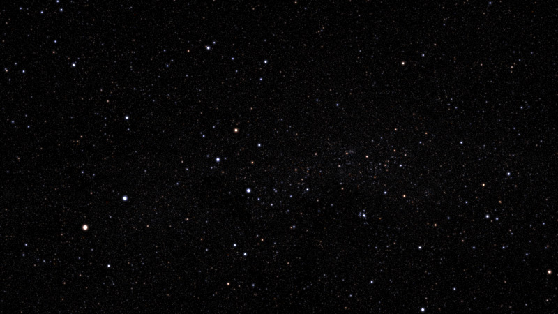
The southern hemisphere Milky Way running east-west through Centaurus, Crux (the Southern Cross, just left of center), and Carina. Alpha Centauri is the bright star in the lower left.
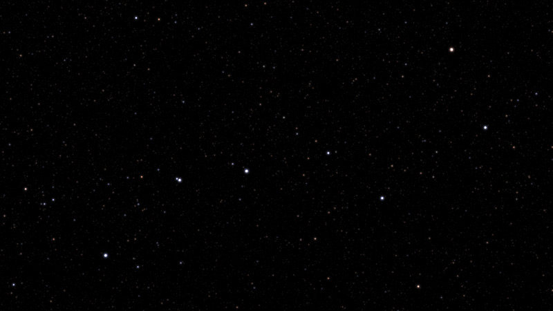
The familiar Big Dipper in Ursa Major, with the bowl on the right and the handle on the left.
The methods and data I've used to create these images have changed considerably over time, as you can see from the following two images of Orion and Taurus from previous versions of this page. I started out by plotting the 9000 or so naked-eye stars in the Yale Bright Star Catalog. Later, I added deeper catalogs for a richer field and started experimenting with varying star sizes to increase the apparent dynamic range. More recently I made the leap to subpixel positional accuracy and more sophisticated modeling of the point spread function.
 Each star in this early image is a single pixel. I assigned the brightest stars
one of four colors (orange, yellow, white, light blue) based on stellar class,
and I used six levels of brightness, one for each stellar magnitude.
Each star in this early image is a single pixel. I assigned the brightest stars
one of four colors (orange, yellow, white, light blue) based on stellar class,
and I used six levels of brightness, one for each stellar magnitude.
This looked pretty good on low-res displays, particularly CRTs, where the device's inherent blur and bloom actually enhanced the effect. It still sort of works, but it's a bit sparse and colorless.
It also doesn't animate well. Because the star positions are quantized onto the pixel grid, camera motions make the stars jitter like an 8-bit video game.
With faster computers and larger drives, it got easier to add as many as a million stars from deeper catalogs. The richer field revealed the outlines of the Milky Way.
In this sea of points, the brightest stars got lost unless I made them bigger. Single pixels don't have enough dynamic range.
But I still can't animate this. In fact, it's a worst case for most animation codecs. From the point of view of an MPEG encoder, it's nothing but high frequency noise, and at practical bit rates, it turns into a shimmering mess.
The third image, scaled to match the other two, shows how I'm rendering star fields now. It may look a bit blurry when put next to the other two, but this is at least partly an image scale problem (your screen doesn't have enough pixels). Each star is drawn in a way that better captures what a camera sees, and it has the added benefit of low-pass filtering the image, which makes animation encoders much happier.
I developed my current method in 2008, while working on my Voyager 1 demo animation, and I continue to refine it as part of my day job.
